How to Freeze Rows and Columns in Google Sheets (and Excel)

When a sheet has hundreds of rows, the header row disappears as soon as you scroll down, and you end up guessing which column is which. Freezing rows or columns keeps them fixed on screen while the rest of the sheet scrolls. It takes two clicks.

Freeze the top row in Google Sheets

Open your spreadsheet. You don't need to select anything.
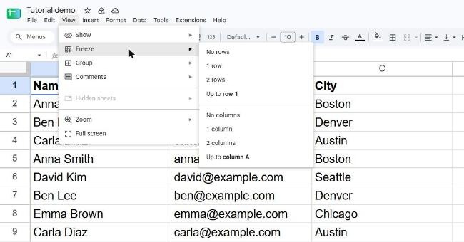
Go to View → Freeze → 1 row.

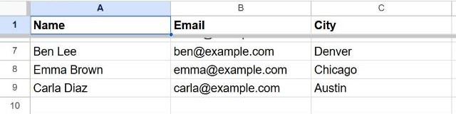
Google Sheets View menu open with Freeze options: No rows, 1 row, 2 rows, Up to row 1, and the same for columns — View → Freeze offers rows and columns in the same menu.

A thicker gray line appears under row 1. Scroll down and your headers stay at the top.

Frozen header row Name, Email, City staying visible above row 7 after scrolling down — After scrolling, the header row stays visible above row 7.

The same menu offers 2 rows if your header takes up two lines.

Freeze several rows

Click any cell in the last row you want to freeze. For example, to freeze rows 1 to 4, click a cell in row 4.
Go to View → Freeze → Up to row 4. The menu shows the number of the row you selected.

Freeze columns

Freezing columns is useful for wide sheets where the first column holds names or IDs.

First column: View → Freeze → 1 column.
Several columns: click a cell in the last column to freeze, then View → Freeze → Up to column C (the letter matches your selection).

You can freeze rows and columns at the same time. For example, freeze 1 row and 1 column to keep both the headers and the name column visible.

The drag shortcut

In the top-left corner of the sheet, above row 1 and left of column A, there are two thick gray bars. Drag the horizontal bar down below the rows you want to freeze, or drag the vertical bar right past the columns you want to freeze. It does exactly the same as the menu.

Unfreeze rows and columns

Go to View → Freeze and choose No rows or No columns. You can also drag the gray bar back to the top-left corner.

Good to know: freezing only affects how the sheet is displayed. It doesn't change your data, formulas or sorting, and everyone who opens the sheet sees the same frozen rows.

How to freeze panes in Excel

Excel calls this feature Freeze Panes and it lives on the View tab of the ribbon:

View → Freeze Panes → Freeze Top Row keeps row 1 visible.
View → Freeze Panes → Freeze First Column keeps column A visible.
To freeze several rows and columns at once, click the cell just below and to the right of what you want to freeze, then choose View → Freeze Panes → Freeze Panes. For example, selecting cell B3 freezes rows 1–2 and column A.

To undo it, go to View → Freeze Panes → Unfreeze Panes.

Frequently asked questions

Why is the Freeze option not doing anything?

If you're scrolled down when you freeze, the frozen area may fill most of the screen. Scroll back to the top first, then freeze. In Google Sheets you also can't freeze more rows than fit on the screen.

Will my frozen header print on every page?

In Google Sheets, yes: when you print or export to PDF, open Headers & footers in the print settings and make sure Repeat frozen rows is ticked. In Excel, set it under Page Layout → Print Titles → Rows to repeat at top.

Does freezing work when I sort or filter?

Yes, and it helps. When you sort with Data → Sort sheet, Sheets leaves frozen rows in place, so your headers don't get mixed into the data.